VLOOKUP by cell background color

 

VLOOKUP by cell background color

In this article you will learn how we can use VLOOKUP by a cell background color. We will create a User Defined Function (UDF) in VBA and will access it on the worksheet. We can use this function when we have to get the value from a table on the base of cell background color is place of lookup value. 

• Copy the below given code and go to Visual Basic Editor (Press Alt+F11)
• Insert a module (Press Alt+I+M)
• Paste this code in the module.
• Save as the workbook as Macro enable workbook.

Function myvlookup(r1 As Range, r2 As Range, n As Integer, a As Boolean) As Variant

Application.Volatile

Dim cel As Range
Dim i As Integer
i = 0
For Each cel In r2
 If cel.Interior.Color = r1.Interior.Color Then
 myvlookup = cel.Offset(0, n - 1).Value
 i = i + 1
 If a = False Then
 Exit For
 End If
 End If

Next

If i = 0 Then myvlookup = "#N/A"


End Function

See the below example:

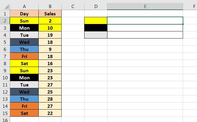
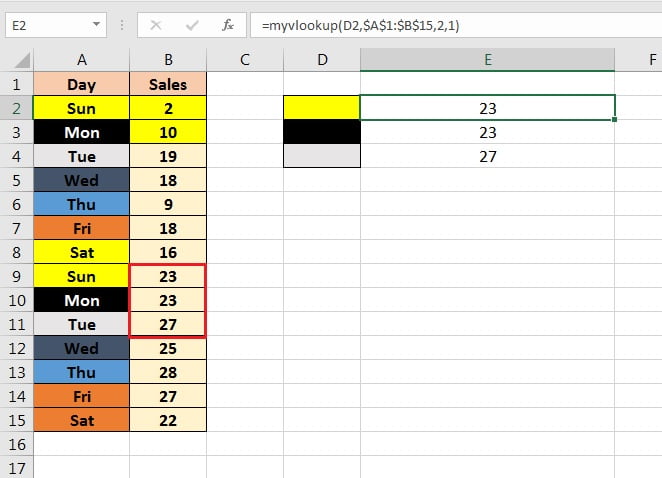
Let’s say we have below given data on Range “A1:B15” and we have to get the sales from column B on Range “E2:E4” on the base of Range “D2:D4” cell background color.

Sale Data

Since we have pasted the above-given code in the module so “myvlookup” function will be available in this workbook now.

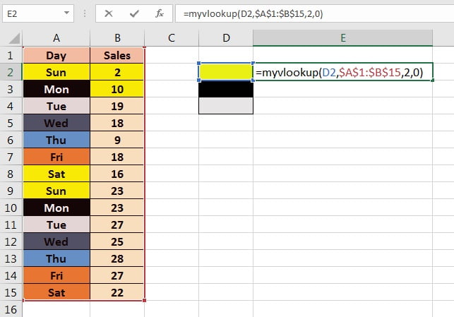
Put the formula =myvlookup(D2,$A$1:$B$15,2,0) on Range “E2”.

myvlookup Function

Fill down the formula till E5.

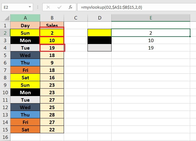
Since we have used 0 (Zero) in our formula “(=myvlookup(D2,$A$1:$B$15,2,0)” so it will give value which will be found first.

As you are seeing in below image value available on column E are the first found values.

myvlookup function with 0

To get the value which is available in the last we need to use 1 in place of 0 in myvlookup formula “(=myvlookup(D2,$A$1:$B$15,2,1)”

myvlookup function with 1

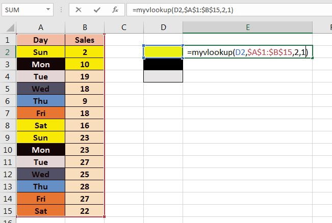
Now we will get the last value for that cell background color.

myvlookup function

Click here to download this excel file.

[Source: Pk-An Excel expart, Google search ]